Note
Click here to download the full example code
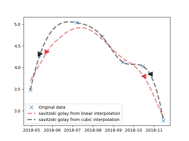
Get phenology metrics
This example shows how to smooth a time series using linear, cubic interpolation or savitzski_golay. Then how to get phenology metrics (start of season, end of season, length of season and amplitude)
import library
import numpy as np
from museopheno import time_series
Create example values
Initially these values came from the LCHloC spectral index
x = np.asarray([3.4825737, 4.27786  , 5.0373, 4.7196426, 4.1233397, 4.0338645,2.7735472])

dates = [20180429, 20180513, 20180708, 20180815, 20180915, 20181015, 20181115]
Resample to every 5 days
dates_5days = time_series.generate_temporal_sampling(dates[0],dates[-1],5)

ts = time_series.SmoothSignal(dates=dates,output_dates = dates_5days)
savitzski golay
# Savitzski golay can use several interpolation type before smoothing the trend
Savitzski golay from linear interpolation
x_savgol_linear = ts.savitzski_golay(x,window_length=9,polyorder=1,interpolation_params=dict(kind='linear'))
Savitzski golay from cubic interpolation
x_savgol_cubic = ts.savitzski_golay(x,window_length=9,polyorder=5,interpolation_params=dict(kind='cubic'))


sos_cub,eos_cub=time_series.get_phenology_metrics(x_savgol_cubic,sos=0.5,eos=0.5)[0]
sos_lin,eos_lin=time_series.get_phenology_metrics(x_savgol_linear,sos=0.5,eos=0.5)[0]
#x_doublelogistic = ts.doubleLogistic(x,t01=10,t02=120)
#sos_dl,eos_dl=time_series.getPhenologyMetrics(x_doublelogistic,sos=0.3,eos=0.8)
#################
# Plot results
from matplotlib import pyplot as plt
plt.plot_date(ts.init_datetime,x,'x',color='C0',markersize=8,label='Original data')

plt.plot_date(ts.output_datetime,x_savgol_linear.flatten(),'--',linewidth=3,color='C3',label='savitzski golay from linear interpolation',alpha=.5)
plt.plot_date(ts.output_datetime,x_savgol_cubic.flatten(),'--',linewidth=3,color='black',label='savitzski golay from cubic interpolation',alpha=.5)
#plt.plot_date(ts.output_datetime,x_doublelogistic.flatten(),'-',linewidth=3,color='C1',label='double logistic',alpha=.5)

plt.plot_date(ts.output_datetime[sos_lin],x_savgol_linear[:,sos_lin],'>',markersize=12,color='C3',alpha=.8)
plt.plot_date(ts.output_datetime[eos_lin],x_savgol_linear[:,eos_lin],'<',markersize=12,color='C3',alpha=.8)

plt.plot_date(ts.output_datetime[sos_cub],x_savgol_cubic[:,sos_cub],'>',markersize=12,color='black',alpha=.8)
plt.plot_date(ts.output_datetime[eos_cub],x_savgol_cubic[:,eos_cub],'<',markersize=12,color='black',alpha=.8)

#plt.plot_date(ts.output_datetime[sos_dl],x_doublelogistic[sos_dl],'>',markersize=12,color='C1',alpha=.8,label='start of season')
#plt.plot_date(ts.output_datetime[eos_dl],x_doublelogistic[eos_dl],'<',markersize=12,color='C1',alpha=.8,label='end of season')


plt.legend(loc='best')
Out:
<matplotlib.legend.Legend object at 0x7f72bd354e90>
Total running time of the script: ( 0 minutes 0.118 seconds)