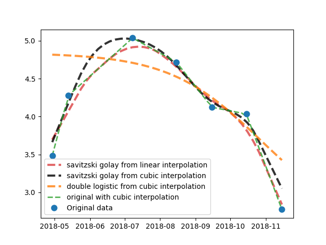
Smooth index or one band time series

This example shows how to smooth a time series using linear, cubic interpolation or savitzski_golay.

import library

import numpy as np
from museopheno import time_series

Create example values

Initially these values came from the LCHloC spectral index

x = np.asarray([3.4825737, 4.27786  , 5.0373, 4.7196426, 4.1233397, 4.0338645,2.7735472])

dates = [20180429, 20180513, 20180708, 20180815, 20180915, 20181015, 20181115]

Resample to every 5 days

dates_5days = time_series.generate_temporal_sampling(dates[0],dates[-1],5)


ts_manager = time_series.SmoothSignal(dates=dates,output_dates = dates_5days)

linear interpolation

x_linear = ts_manager.interpolation(x,kind='linear')
print(x_linear)

Out:

[[3.4825737  3.76660452 4.05063534 4.29142143 4.35922857 4.42703571
  4.49484286 4.56265    4.63045714 4.69826429 4.76607143 4.83387857
  4.90168571 4.96949286 5.0373     4.99550297 4.95370595 4.91190892
  4.87011189 4.82831487 4.78651784 4.74472082 4.68117145 4.58499356
  4.48881567 4.39263778 4.2964599  4.20028201 4.12035719 4.10544466
  4.09053213 4.07561959 4.06070706 4.04579453 3.9932091  3.78993212
  3.58665514 3.38337815 3.18010117 2.97682418 2.7735472 ]]

cubic interpolation

x_cubic = ts_manager.interpolation(x,kind='cubic')
print(x_cubic)

Out:

[[3.4825737  3.80799141 4.08649468 4.32156729 4.516693   4.67535558
  4.80103881 4.89722644 4.96740226 5.01505002 5.0436535  5.05669647
  5.0576627  5.05003595 5.0373     5.02198591 5.00281393 4.97755161
  4.94396649 4.89982614 4.84289809 4.77094989 4.68186017 4.57782569
  4.46665263 4.35652206 4.25561504 4.17211263 4.11417114 4.08469853
  4.07489294 4.07436811 4.07273781 4.05961576 4.02461571 3.95735141
  3.84743661 3.68448504 3.45811045 3.15792659 2.7735472 ]]

savitzski golay

# Savitzski golay can use several interpolation type before smoothing the trend

Savitzski golay from linear interpolation

x_savgol_linear = ts_manager.savitzski_golay(x,window_length=9,polyorder=1,interpolation_params=dict(kind='linear'))

Savitzski golay from cubic interpolation

x_savgol_cubic = ts_manager.savitzski_golay(x,window_length=9,polyorder=1,interpolation_params=dict(kind='cubic'))

x_doublelogistic = ts_manager.double_logistic(x)


#################
# Plot results
from matplotlib import pyplot as plt
plt.plot_date(ts_manager.output_datetime,x_savgol_linear.flatten(),'--',linewidth=3,color='C3',label='savitzski golay from linear interpolation',alpha=.7)
plt.plot_date(ts_manager.output_datetime,x_savgol_cubic.flatten(),'--',linewidth=3,color='black',label='savitzski golay from cubic interpolation',alpha=.8)

plt.plot_date(ts_manager.output_datetime,x_doublelogistic.flatten(),'--',linewidth=3,color='C1',label='double logistic from cubic interpolation',alpha=.8)

plt.plot_date(ts_manager.output_datetime,x_linear.flatten(),'--',linewidth=2,color='C2',label='original with cubic interpolation',alpha=.8)

plt.plot_date(ts_manager.init_datetime,x,'o',color='C0',markersize=8,label='Original data')
plt.legend(loc='best')

Out:

/home/docs/checkouts/readthedocs.org/user_builds/museopheno/checkouts/develop/museopheno/time_series/__dl.py:58: RuntimeWarning: overflow encountered in square
  df[4, :] = A / x3 * np.exp((x2-t)/x3) * 1/(1+np.exp((x2-t)/x3))**2
/home/docs/checkouts/readthedocs.org/user_builds/museopheno/checkouts/develop/museopheno/time_series/__dl.py:61: RuntimeWarning: overflow encountered in square
  df[5, :] = -A * (x2 - t) / x3**2 * np.exp((x2-t)/x3) * 1/(1+np.exp((x2-t)/x3))**2
/home/docs/checkouts/readthedocs.org/user_builds/museopheno/checkouts/develop/museopheno/time_series/__dl.py:27: RuntimeWarning: overflow encountered in exp
  f2 = 1/(1+np.exp((x2-t)/x3))
/home/docs/checkouts/readthedocs.org/user_builds/museopheno/checkouts/develop/museopheno/time_series/__dl.py:46: RuntimeWarning: overflow encountered in exp
  df[0, :] = 1/(1+np.exp((x0-t)/x1)) - 1/(1+np.exp((x2-t)/x3))
/home/docs/checkouts/readthedocs.org/user_builds/museopheno/checkouts/develop/museopheno/time_series/__dl.py:58: RuntimeWarning: overflow encountered in exp
  df[4, :] = A / x3 * np.exp((x2-t)/x3) * 1/(1+np.exp((x2-t)/x3))**2
/home/docs/checkouts/readthedocs.org/user_builds/museopheno/checkouts/develop/museopheno/time_series/__dl.py:58: RuntimeWarning: invalid value encountered in true_divide
  df[4, :] = A / x3 * np.exp((x2-t)/x3) * 1/(1+np.exp((x2-t)/x3))**2
/home/docs/checkouts/readthedocs.org/user_builds/museopheno/checkouts/develop/museopheno/time_series/__dl.py:61: RuntimeWarning: overflow encountered in exp
  df[5, :] = -A * (x2 - t) / x3**2 * np.exp((x2-t)/x3) * 1/(1+np.exp((x2-t)/x3))**2
/home/docs/checkouts/readthedocs.org/user_builds/museopheno/checkouts/develop/museopheno/time_series/__dl.py:61: RuntimeWarning: invalid value encountered in true_divide
  df[5, :] = -A * (x2 - t) / x3**2 * np.exp((x2-t)/x3) * 1/(1+np.exp((x2-t)/x3))**2

<matplotlib.legend.Legend object at 0x7f72bd3d5510>