Compute Leaf Chlorophyll Content from S2 Time Series

This example shows how to compute an index (here LChloC) from a S2 with 10 bands. The raster is order date per date (blue,green,red…date 1 then blue,green,red… date 2…)

Import libraries

import numpy as np
from museopheno import sensors,datasets

Import raster dataset with list of dates

raster,dates = datasets.Sentinel2_3a_2018(return_dates=True)

Create an instance of sensors.Sentinel2 with 10bands

S2 = sensors.Sentinel2(n_bands=10)

print('Default band order for 10 bands is : '+', '.join(S2.bands_order)+'.')

# List of available index :
S2.available_indices.keys()

Out:

Default band order for 10 bands is : 2, 3, 4, 8, 5, 6, 7, 8A, 11, 12.

dict_keys(['B2', 'B3', 'B4', 'B8', 'B5', 'B6', 'B7', 'B8A', 'B11', 'B12', 'ACORVI', 'ACORVInarrow', 'SAVI', 'EVI', 'EVI2', 'PSRI', 'ARI', 'ARI2', 'MARI', 'CHLRE', 'MCARI', 'MSI', 'MSIB12', 'NDrededgeSWIR', 'SIPI2', 'NDWI', 'LCaroC', 'LChloC', 'LAnthoC', 'Chlogreen', 'NDRESWIR', 'NDVI', 'NDVInarrow', 'NDVIre', 'RededgePeakArea', 'Rratio', 'MTCI', 'S2REP', 'IRECI', 'NBR', 'REP', 'WDRVI_B6B7'])

Write metadata in each band (date + band name)

Write metadata in each band (date + band name) in order to use raster timeseries manager plugin on QGIS or to have the date and the band in the list of bands QGIS.

S2.set_description_metadata(raster,dates)

Generate index from array

X = datasets.Sentinel2_3a_2018(return_random_sample=True)
LChloC = S2.generate_index(X,S2.get_index_expression('LChloC'),dtype=np.float32)
print(LChloC)

Out:

Total number of blocks : 1
[[4.744658  5.721198  6.9290657 ... 6.244186  5.810757  2.6099865]
 [4.744658  5.721198  6.9290657 ... 6.244186  5.810757  2.6099865]
 [4.670705  5.5403867 7.318949  ... 6.091858  5.764454  2.7043796]
 ...
 [4.971503  6.7136    7.456     ... 5.7030964 5.3644524 2.3870163]
 [4.971503  6.7136    7.456     ... 5.7030964 5.3644524 2.3870163]
 [5.162269  6.9686985 7.631579  ... 5.7843137 5.5149913 2.3586957]]

Generate index from and to a raster

S2.generate_raster(input_raster=raster,output_raster='/tmp/LChloC.tif',expression=S2.get_index_expression('LChloC'),dtype=np.float32)

Out:

Total number of blocks : 1
Using datatype from numpy table : float32.
Detected 7 bands for function expression_manager.
Batch processing (1 blocks using 11Mo of ram)

Computing index [########################################]100%

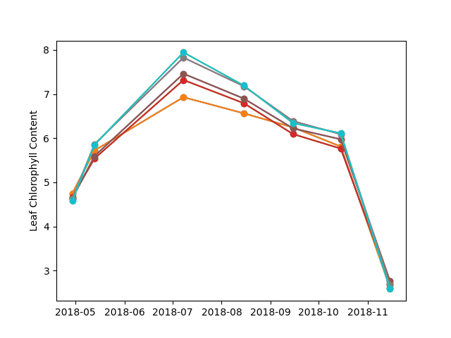
Plot example of LChloC

from matplotlib import pyplot as plt
from datetime import datetime
dateToDatetime = [datetime.strptime(str(date),'%Y%m%d') for date in dates]
plt.plot_date(dateToDatetime,LChloC[:10,:].T,'-o')
plt.ylabel('Leaf Chlorophyll Content')
import os
os.remove('/tmp/LChloC.tif')