Note
Click here to download the full example code
Add or modify an spectral index of a sensor
This example shows how to add or modify an index for a specific sensor. Here we add/modify the NBR index (Normalized Burn-Ratio), then we generate a raster.
Import libraries
import numpy as np
from museopheno import sensors,datasets
Import dataset
X,dates = datasets.Sentinel2_3a_2018(return_dates=True,return_random_sample=True)

S2 = sensors.Sentinel2(n_bands=10)

print('Default band order for 10 bands is : '+', '.join(S2.bands_order)+'.')
Out:
Total number of blocks : 1
Default band order for 10 bands is : 2, 3, 4, 8, 5, 6, 7, 8A, 11, 12.
Look at available S2 index
S2.available_indices
Out:
{'B2': {'expression': 'B2'}, 'B3': {'expression': 'B3'}, 'B4': {'expression': 'B4'}, 'B8': {'expression': 'B8'}, 'B5': {'expression': 'B5'}, 'B6': {'expression': 'B6'}, 'B7': {'expression': 'B7'}, 'B8A': {'expression': 'B8A'}, 'B11': {'expression': 'B11'}, 'B12': {'expression': 'B12'}, 'ACORVI': {'expression': '( B8 - B4 + 0.05 ) / ( B8 + B4 + 0.05 ) ', 'condition': '(B8+B4+0.05) != 0'}, 'ACORVInarrow': {'expression': '( B8A - B4 + 0.05 ) / ( B8A + B4 + 0.05 ) ', 'condition': '(B8A+B4+0.05) != 0'}, 'SAVI': {'expression': ['1.5 * (B8 - B4) / ( B8 + B4 + 0.5 )']}, 'EVI': {'expression': ['( 2.5 * ( B8 - B4 ) ) / ( ( B8 + 6 * B4 - 7.5 * B2 ) + 1 )']}, 'EVI2': {'expression': '( 2.5 * (B8 - B4) ) / (B8 + 2.4 * B4 + 1) ', 'condition': 'B8+2.4*B4+1 != 0'}, 'PSRI': {'expression': '( (B4 - B2) / B5 )', 'condition': 'B5 != 0'}, 'ARI': {'expression': '( 1 / B3 ) - ( 1 / B5 )', 'condition': 'np.logical_and(B3 != 0, B5 != 0)'}, 'ARI2': {'expression': '( B8 / B2 ) - ( B8 / B3 )', 'condition': ' np.logical_and(B2 != 0, B3 != 0)'}, 'MARI': {'expression': '( (B5 - B5 ) - 0.2 * (B5 - B3) ) * (B5 / B4)', 'condition': 'B4 != 0'}, 'CHLRE': {'expression': 'np.power(B5 / B7,-1.0)', 'condition': 'B5!=0'}, 'MCARI': {'expression': ' ( ( B5 - B4 ) - 0.2 * ( B5 - B3 ) ) * ( B5 / B4 )', 'condition': 'B4 != 0'}, 'MSI': {'expression': 'B11 / B8', 'condition': 'B8 != 0'}, 'MSIB12': {'expression': 'B12 / B8', 'condition': 'B8 != 0'}, 'NDrededgeSWIR': {'expression': '( B6 - B12 ) / ( B6 + B12 )', 'condition': '( B6 + B12 ) != 0'}, 'SIPI2': {'expression': '( B8 - B3 ) / ( B8 - B4 )', 'condition': 'B8 - B4 != 0'}, 'NDWI': {'expression': '(B8-B11)/(B8+B11)', 'condition': '(B8+B11) != 0'}, 'LCaroC': {'expression': 'B7 / ( B2-B5 )', 'condition': '( B7 ) != 0'}, 'LChloC': {'expression': 'B7 / B5', 'condition': 'B5 != 0'}, 'LAnthoC': {'expression': 'B7 / (B3 - B5) ', 'condition': '( B3-B5 ) !=0'}, 'Chlogreen': {'expression': ['B8A / (B3 + B5)']}, 'NDRESWIR': {'expression': '(B6-B12)/(B6+B12)', 'condition': '(B6+B12) != 0'}, 'NDVI': {'expression': '(B8-B4)/(B8+B4)', 'condition': '(B8+B4) != 0'}, 'NDVInarrow': {'expression': '(B8A-B4)/(B8A+B4)', 'condition': '(B8A+B4) != 0'}, 'NDVIre': {'expression': '(B8A-B5)/(B8A+B5)', 'condition': '(B8A+B5) != 0'}, 'RededgePeakArea': {'expression': ['B4+B5+B6+B7+B8A']}, 'Rratio': {'expression': ['B4/(B2+B3+B4)']}, 'MTCI': {'expression': '(B6 - B5)/(B5 - B4)', 'condition': '(B5-B4) != 0'}, 'S2REP': {'expression': ['35 * ((((B7 + B4)/2) - B5)/(B6 - B5))']}, 'IRECI': {'expression': '(B7-B4)/(B5/B6)', 'condition': 'np.logical_and(B5 != 0, B6 != 0)'}, 'NBR': {'expression': '(B08 - B12) / (B08 + B12)', 'condition': '(B08+B12)!=0'}, 'REP': {'expression': ['700 + 40 * (( ( B4 + B7 ) / B2) -5) / ( B6 - B5 ) ']}, 'WDRVI_B6B7': {'expression': '(0.1*B7+B6) / (0.1*B7-B6)', 'condition': ' (0.1*B7-B6) != 0'}}
add the NBR index
This index is already in MuseoPheno, but if you change the expression it will overwrite the previous one
S2.add_index('NBR',expression='(B08 - B12) / (B08 + B12)',condition='(B08+B12)!=0')
compute NBR from an array
NBR = S2.generate_index(X,S2.get_index_expression('NBR'))
Produce the index raster
# We multiply by 100 to save with int16 datatype
raster = datasets.Sentinel2_3a_2018()
S2.generate_raster(raster,output_raster='/tmp/NBR.tif',expression=S2.get_index_expression('NBR'),multiply_by=100,dtype=np.int16)
###################
# plot result
from matplotlib import pyplot as plt
from datetime import datetime
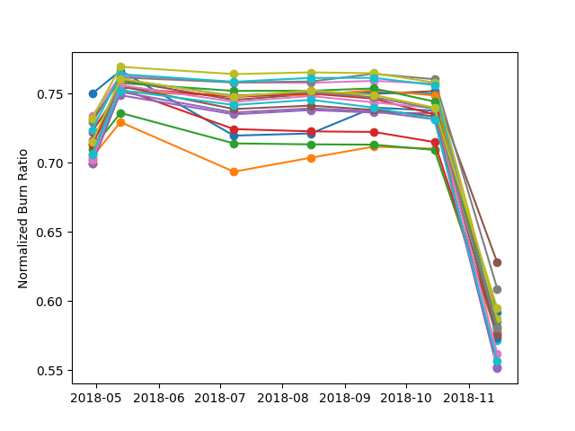
dateToDatetime = [datetime.strptime(str(date),'%Y%m%d') for date in dates]
plt.plot_date(dateToDatetime,NBR[:20,:].T,'-o')
plt.ylabel('Normalized Burn Ratio')
Out:
Total number of blocks : 1
Using datatype from numpy table : int16.
Detected 7 bands for function expression_manager.
Batch processing (1 blocks using 10Mo of ram)

Computing index [########################################]100%

Text(0, 0.5, 'Normalized Burn Ratio')
Total running time of the script: ( 0 minutes 2.280 seconds)