Note
Click here to download the full example code
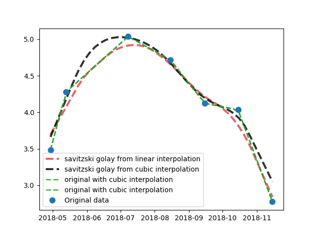
Smooth times series with different spectral bands
This example shows how to smooth a time series using linear, cubic interpolation or savitzski_golay.
import library
import numpy as np
from museopheno import time_series
Create example values
Initially these values came from the LCHloC spectral index
x = np.asarray([3.4825737, 4.27786  , 5.0373, 4.7196426, 4.1233397, 4.0338645,2.7735472])
x = np.hstack((x,x*1.3)) # simulate two different bands ordered by date [b1,b2...] then [b1,b2...]
dates = [20180429, 20180513, 20180708, 20180815, 20180915, 20181015, 20181115]
Resample to every 5 days
dates_5days = time_series.generate_temporal_sampling(dates[0],dates[-1],5)


ts = time_series.SmoothSignal(dates=dates,output_dates = dates_5days,bands_order=['B1','B2'],order_by='band')
linear interpolation
x_linear = ts.interpolation(x,kind='linear')
print(x_linear)
Out:
[[3.4825737  3.76660452 4.05063534 4.29142143 4.35922857 4.42703571
  4.49484286 4.56265    4.63045714 4.69826429 4.76607143 4.83387857
  4.90168571 4.96949286 5.0373     4.99550297 4.95370595 4.91190892
  4.87011189 4.82831487 4.78651784 4.74472082 4.68117145 4.58499356
  4.48881567 4.39263778 4.2964599  4.20028201 4.12035719 4.10544466
  4.09053213 4.07561959 4.06070706 4.04579453 3.9932091  3.78993212
  3.58665514 3.38337815 3.18010117 2.97682418 2.7735472  4.52734581
  4.89658588 5.26582595 5.57884786 5.66699714 5.75514643 5.84329571
  5.931445   6.01959429 6.10774357 6.19589286 6.28404214 6.37219143
  6.46034071 6.54849    6.49415387 6.43981773 6.3854816  6.33114546
  6.27680933 6.22247319 6.16813706 6.08552288 5.96049163 5.83546037
  5.71042912 5.58539787 5.46036661 5.35646435 5.33707806 5.31769176
  5.29830547 5.27891918 5.25953288 5.19117183 4.92691176 4.66265168
  4.3983916  4.13413152 3.86987144 3.60561136]]
cubic interpolation
x_cubic = ts.interpolation(x,kind='cubic')
print(x_cubic)
Out:
[[3.4825737  3.80799141 4.08649468 4.32156729 4.516693   4.67535558
  4.80103881 4.89722644 4.96740226 5.01505002 5.0436535  5.05669647
  5.0576627  5.05003595 5.0373     5.02198591 5.00281393 4.97755161
  4.94396649 4.89982614 4.84289809 4.77094989 4.68186017 4.57782569
  4.46665263 4.35652206 4.25561504 4.17211263 4.11417114 4.08469853
  4.07489294 4.07436811 4.07273781 4.05961576 4.02461571 3.95735141
  3.84743661 3.68448504 3.45811045 3.15792659 2.7735472  4.52734581
  4.95038883 5.31244309 5.61803748 5.8717009  6.07796226 6.24135045
  6.36639438 6.45762294 6.51956503 6.55674956 6.57370542 6.57496151
  6.56504674 6.54849    6.52858168 6.50365811 6.47081709 6.42715644
  6.36977398 6.29576751 6.20223486 6.08641822 5.9511734  5.80664842
  5.66347868 5.53229955 5.42374642 5.34842249 5.31010809 5.29736082
  5.29667855 5.29455915 5.27750048 5.23200042 5.14455684 5.00166759
  4.78983055 4.49554359 4.10530457 3.60561136]]
savitzski golay
# Savitzski golay can use several interpolation type before smoothing the trend
Savitzski golay from linear interpolation
x_savgol_linear = ts.savitzski_golay(x,window_length=9,polyorder=1,interpolation_params=dict(kind='linear'))
Savitzski golay from cubic interpolation
x_savgol_cubic = ts.savitzski_golay(x,window_length=9,polyorder=1,interpolation_params=dict(kind='cubic'))


#################
# Plot results
from matplotlib import pyplot as plt
plt.plot_date(ts.output_datetime,x_savgol_linear.flatten()[:len(dates_5days)],'--',linewidth=3,color='C3',label='savitzski golay from linear interpolation',alpha=.7)
plt.plot_date(ts.output_datetime,x_savgol_cubic.flatten()[:len(dates_5days)],'--',linewidth=3,color='black',label='savitzski golay from cubic interpolation',alpha=.8)

plt.plot_date(ts.output_datetime,x_linear.flatten()[:len(dates_5days)],'--',linewidth=2,color='C2',label='original with cubic interpolation',alpha=.8)
plt.plot(ts.output_datetime,x_linear.flatten()[:len(dates_5days)],'--',linewidth=2,color='C2',label='original with cubic interpolation',alpha=.8)

plt.plot_date(ts.init_datetime,x[:int(x.shape[0]/2)],'o',color='C0',markersize=8,label='Original data')
plt.legend(loc='best')
Out:
<matplotlib.legend.Legend object at 0x7fafb6364710>
Total running time of the script: ( 0 minutes 0.157 seconds)